de Kaggle
Introducción
El dataset de supervivientes a la catástrofe de Titanic es un sujeto clásico para el ingreso al mundo de Machine Learning, casi el "Hola Mundo" del área. Este set tiene una amplia gama de datos diferentes con sus peculiaridades que lo hacen un conjunto variado y que permite tocar varias áreas del proceso de Machine Learning. En este estudio del caso tratemos de predecir si una persona sobreviviría la catástrofe del Titanic dadas sus características previas al accidente, y con esto una demo de herramientas de Python que podemos usar para Machine Learning.
Agregamos los imports necesarios
Numpy y Pandas los usaremos para las operaciones y manipulación de datos.
Seaborn y Matplotlib es para graficado.
Warnings y os lo usaremos para ver el directorio de inputs.
import numpy as np
import pandas as pd

import seaborn as sns
from matplotlib import pyplot as plt
sns.set_style("whitegrid")
%matplotlib inline

import warnings
warnings.filterwarnings("ignore")

import os
print(os.listdir("./input"))
['gender_submission.csv', 'test.csv', 'train.csv']
Vamos a estar utilizando los dataset de Titanic, que ya hemos visto previamente. Tenemos el set ya particionado para test y entrenamiento de modelos, aparte de uno donde se presume que todas y solamente las mujeres sobreviven.
Cargamos y evaluamos nuestros datos
Con pandas podemos importar los datos, ver algunos valores y estadísticas generales muy fácilmente.
trainingData = pd.read_csv("./input/train.csv")
testData = pd.read_csv("./input/test.csv")

trainingData.head()
| PassengerId | Survived | Pclass | Name | Sex | Age | SibSp | Parch | Ticket | Fare | Cabin | Embarked | |
|---|---|---|---|---|---|---|---|---|---|---|---|---|
| 0 | 1 | 0 | 3 | Braund, Mr. Owen Harris | male | 22.0 | 1 | 0 | A/5 21171 | 7.2500 | NaN | S |
| 1 | 2 | 1 | 1 | Cumings, Mrs. John Bradley (Florence Briggs Th... | female | 38.0 | 1 | 0 | PC 17599 | 71.2833 | C85 | C |
| 2 | 3 | 1 | 3 | Heikkinen, Miss. Laina | female | 26.0 | 0 | 0 | STON/O2. 3101282 | 7.9250 | NaN | S |
| 3 | 4 | 1 | 1 | Futrelle, Mrs. Jacques Heath (Lily May Peel) | female | 35.0 | 1 | 0 | 113803 | 53.1000 | C123 | S |
| 4 | 5 | 0 | 3 | Allen, Mr. William Henry | male | 35.0 | 0 | 0 | 373450 | 8.0500 | NaN | S |
trainingData.describe()
| PassengerId | Survived | Pclass | Age | SibSp | Parch | Fare | |
|---|---|---|---|---|---|---|---|
| count | 891.000000 | 891.000000 | 891.000000 | 714.000000 | 891.000000 | 891.000000 | 891.000000 |
| mean | 446.000000 | 0.383838 | 2.308642 | 29.699118 | 0.523008 | 0.381594 | 32.204208 |
| std | 257.353842 | 0.486592 | 0.836071 | 14.526497 | 1.102743 | 0.806057 | 49.693429 |
| min | 1.000000 | 0.000000 | 1.000000 | 0.420000 | 0.000000 | 0.000000 | 0.000000 |
| 25% | 223.500000 | 0.000000 | 2.000000 | 20.125000 | 0.000000 | 0.000000 | 7.910400 |
| 50% | 446.000000 | 0.000000 | 3.000000 | 28.000000 | 0.000000 | 0.000000 | 14.454200 |
| 75% | 668.500000 | 1.000000 | 3.000000 | 38.000000 | 1.000000 | 0.000000 | 31.000000 |
| max | 891.000000 | 1.000000 | 3.000000 | 80.000000 | 8.000000 | 6.000000 | 512.329200 |
Podemos ver ya que hay datos incorrectos, por ejemplo la cabina. Deberemos procesarlos luego. Veamos que otros datos están mal y que tantos.
Pandas nos permite contar cuantos datos son nulos:
pd.isnull(trainingData).sum()
PassengerId      0
Survived         0
Pclass           0
Name             0
Sex              0
Age            177
SibSp            0
Parch            0
Ticket           0
Fare             0
Cabin          687
Embarked         2
dtype: int64
pd.isnull(testData).sum()
PassengerId      0
Pclass           0
Name             0
Sex              0
Age             86
SibSp            0
Parch            0
Ticket           0
Fare             1
Cabin          327
Embarked         0
dtype: int64
Cabin tiene muchos nulos, pero podríamos considerarlo un atributo no muy influyente para lo que queremos predecir (los supervivientes), por lo que puede ser util eliminarlo completamente. Ticket también entra en este caso, por lo que lo dropeamos.
trainingData.drop(labels=["Cabin", "Ticket"], axis=1, inplace=True)
testData.drop(labels=["Cabin", "Ticket"], axis=1, inplace=True)
pd.isnull(trainingData).sum()
PassengerId      0
Survived         0
Pclass           0
Name             0
Sex              0
Age            177
SibSp            0
Parch            0
Fare             0
Embarked         2
dtype: int64
Podemos ver que el campo edad también tiene muchos nulos, pero es un dato importante por lo que eliminarlo como atributo es mala idea. Veremos su distribución general para decidir como proseguir con este campo.
copy = trainingData.copy()
copy.dropna(inplace = True)
sns.distplot(copy["Age"])
<Axes: xlabel='Age', ylabel='Density'>
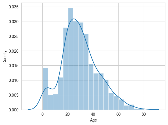
Se denota que las edades son en general un poco mayores, tirando a la derecha en el gráfico. Para los datos faltantes podemos utilizar la media o la mediana. Debido a que los datos favorecen levemente un lado, la mediana es más objetiva.
trainingData["Age"].fillna(trainingData["Age"].median(), inplace = True)
testData["Age"].fillna(testData["Age"].median(), inplace = True)
trainingData["Embarked"].fillna("S", inplace = True)
testData["Fare"].fillna(testData["Fare"].median(), inplace = True)

copy = trainingData.copy()
copy.dropna(inplace = True)
sns.distplot(copy["Age"])
<Axes: xlabel='Age', ylabel='Density'>
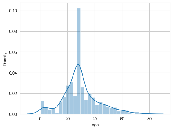
Puede verse intrusivo, pero permite mantener los datos lo más constantes con los originales posible.
Graficando los datos
Graficando y comparando las relaciones de los datos con lo que buscamos predecir nos dará mejor idea de las estructuras subyacentes y facilitará construir el mejor modelo posible para el problema, descartando variables que no inciden en el resultado o que son demasiado correlacionadas. Por ejemplo veamos género y si la persona sobrevivió.
sns.barplot(x="Sex", y="Survived", data=trainingData)
plt.title("Distribution of Survival based on Gender")
plt.show()

total_survived_females = trainingData[trainingData.Sex == "female"]["Survived"].sum()
total_survived_males = trainingData[trainingData.Sex == "male"]["Survived"].sum()

print("Total people survived is: " + str((total_survived_females + total_survived_males)))
print("Proportion of Females who survived:")
print(total_survived_females/(total_survived_females + total_survived_males))
print("Proportion of Males who survived:")
print(total_survived_males/(total_survived_females + total_survived_males))
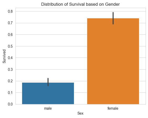
Total people survived is: 342
Proportion of Females who survived:
0.6812865497076024
Proportion of Males who survived:
0.31871345029239767
Al ver la fuerte diferencia entre las proporciones de supervivencia entre los géneros.
Veamos para otros atributos
sns.barplot(x="Pclass", y="Survived", data=trainingData)
plt.ylabel("Survival Rate")
plt.title("Distribution of Survival Based on Class")
plt.show()

total_survived_one = trainingData[trainingData.Pclass == 1]["Survived"].sum()
total_survived_two = trainingData[trainingData.Pclass == 2]["Survived"].sum()
total_survived_three = trainingData[trainingData.Pclass == 3]["Survived"].sum()
total_survived_class = total_survived_one + total_survived_two + total_survived_three

print("Total people survived is: " + str(total_survived_class))
print("Proportion of Class 1 Passengers who survived:")
print(total_survived_one/total_survived_class)
print("Proportion of Class 2 Passengers who survived:")
print(total_survived_two/total_survived_class)
print("Proportion of Class 3 Passengers who survived:")
print(total_survived_three/total_survived_class)
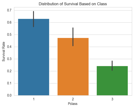
Total people survived is: 342
Proportion of Class 1 Passengers who survived:
0.39766081871345027
Proportion of Class 2 Passengers who survived:
0.2543859649122807
Proportion of Class 3 Passengers who survived:
0.347953216374269
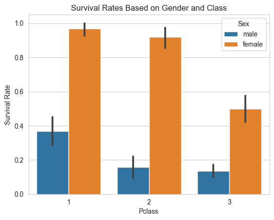
sns.barplot(x="Pclass", y="Survived", hue="Sex", data=trainingData)
plt.ylabel("Survival Rate")
plt.title("Survival Rates Based on Gender and Class")
Text(0.5, 1.0, 'Survival Rates Based on Gender and Class')
sns.barplot(x="Sex", y="Survived", hue="Pclass", data=trainingData)
plt.ylabel("Survival Rate")
plt.title("Survival Rates Based on Gender and Class")
Text(0.5, 1.0, 'Survival Rates Based on Gender and Class')
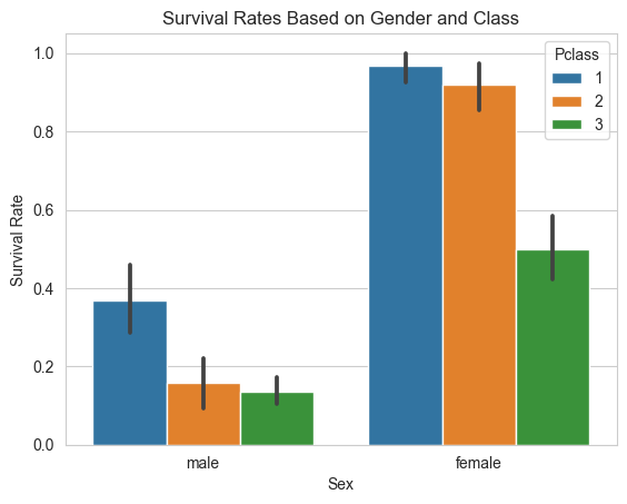
Las diferencias de supervivencia entre las primera y las otras clases es significativa también.
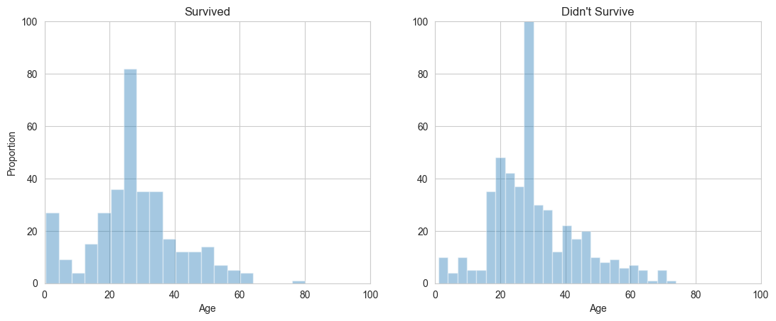
survived_ages = trainingData[trainingData.Survived == 1]["Age"]
not_survived_ages = trainingData[trainingData.Survived == 0]["Age"]
plt.subplot(1, 2, 1)
sns.distplot(survived_ages, kde=False)
plt.axis([0, 100, 0, 100])
plt.title("Survived")
plt.ylabel("Proportion")
plt.subplot(1, 2, 2)
sns.distplot(not_survived_ages, kde=False)
plt.axis([0, 100, 0, 100])
plt.title("Didn't Survive")
plt.subplots_adjust(right=1.7)
plt.show()
sns.stripplot(x="Survived", y="Age", data=trainingData, jitter=True)
<Axes: xlabel='Survived', ylabel='Age'>
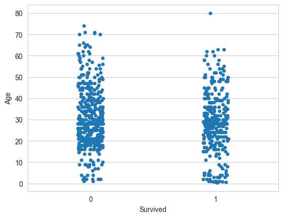
Podemos ver concentraciones excepcionales de supervivientes en los menores de edad respecto a los que perecieron.
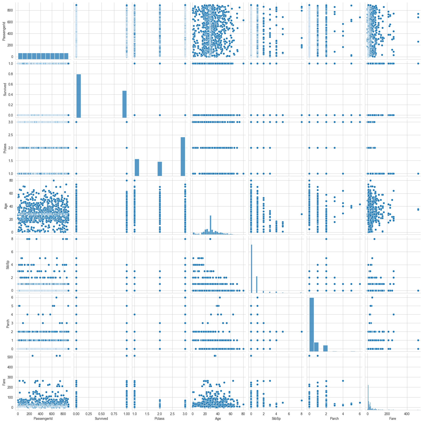
si queremos ver todos los datos y como se relacionan, se puede crear con el siguiente comando:
sns.pairplot(trainingData)
<seaborn.axisgrid.PairGrid at 0x2278ce93970>
Feature Engineering
Pasaremos a procesar y adaptar nuestros atributos a formas más manejables. Para nuestro caso debemos convertir todos los datos a numéricos, ya que solo estos puede tomar el modelo.
Por ejemplo datos categóricos como género o embarcó.
Usaremos One-Hot-Encoding por sklearn
set(trainingData["Sex"])
{'female', 'male'}
set(trainingData["Embarked"])
{'C', 'Q', 'S'}
from sklearn.preprocessing import LabelEncoder

le_sex = LabelEncoder()
le_sex.fit(trainingData["Sex"])

encoded_sex_training = le_sex.transform(trainingData["Sex"])
trainingData["Sex"] = encoded_sex_training
encoded_sex_testing = le_sex.transform(testData["Sex"])
testData["Sex"] = encoded_sex_testing

le_embarked = LabelEncoder()
le_embarked.fit(trainingData["Embarked"])

encoded_embarked_training = le_embarked.transform(trainingData["Embarked"])
trainingData["Embarked"] = encoded_embarked_training
encoded_embarked_testing = le_embarked.transform(testData["Embarked"])
testData["Embarked"] = encoded_embarked_testing

#vemos el resultado
trainingData.sample(5)
| PassengerId | Survived | Pclass | Name | Sex | Age | SibSp | Parch | Fare | Embarked | |
|---|---|---|---|---|---|---|---|---|---|---|
| 764 | 765 | 0 | 3 | Eklund, Mr. Hans Linus | 1 | 16.0 | 0 | 0 | 7.775 | 2 |
| 425 | 426 | 0 | 3 | Wiseman, Mr. Phillippe | 1 | 28.0 | 0 | 0 | 7.250 | 2 |
| 187 | 188 | 1 | 1 | Romaine, Mr. Charles Hallace ("Mr C Rolmane") | 1 | 45.0 | 0 | 0 | 26.550 | 2 |
| 723 | 724 | 0 | 2 | Hodges, Mr. Henry Price | 1 | 50.0 | 0 | 0 | 13.000 | 2 |
| 56 | 57 | 1 | 2 | Rugg, Miss. Emily | 0 | 21.0 | 0 | 0 | 10.500 | 2 |
Podemos también combinar y crear columnas nuevas, por ejemplo unir "número de hermanos y pareja" y "número de padres e hijos" en un solo atributo "familia a bordo", y de este también podemos crear una para saber si alguien viaja solo.
trainingData["FamSize"] = trainingData["SibSp"] + trainingData["Parch"] + 1
testData["FamSize"] = testData["SibSp"] + testData["Parch"] + 1

trainingData["IsAlone"] = trainingData.FamSize.apply(lambda x: 1 if x == 1 else 0)
testData["IsAlone"] = testData.FamSize.apply(lambda x: 1 if x == 1 else 0)

trainingData.sample(5)
| PassengerId | Survived | Pclass | Name | Sex | Age | SibSp | Parch | Fare | Embarked | FamSize | IsAlone | |
|---|---|---|---|---|---|---|---|---|---|---|---|---|
| 601 | 602 | 0 | 3 | Slabenoff, Mr. Petco | 1 | 28.0 | 0 | 0 | 7.8958 | 2 | 1 | 1 |
| 481 | 482 | 0 | 2 | Frost, Mr. Anthony Wood "Archie" | 1 | 28.0 | 0 | 0 | 0.0000 | 2 | 1 | 1 |
| 110 | 111 | 0 | 1 | Porter, Mr. Walter Chamberlain | 1 | 47.0 | 0 | 0 | 52.0000 | 2 | 1 | 1 |
| 319 | 320 | 1 | 1 | Spedden, Mrs. Frederic Oakley (Margaretta Corn... | 0 | 40.0 | 1 | 1 | 134.5000 | 0 | 3 | 0 |
| 369 | 370 | 1 | 1 | Aubart, Mme. Leontine Pauline | 0 | 24.0 | 0 | 0 | 69.3000 | 0 | 1 | 1 |
Otro atributo que podemos calcular es utilizando el nombre. Sin saber el género de la persona, pero si su nombre esta precedido por Mr. o Mrs. entre otros, podemos inferir su género, lo cual es influyente en el resultado. Usaremos encoding similar a como hicimos con embarked y sex.
for name in trainingData["Name"]:
    trainingData["Title"] = trainingData["Name"].str.extract("([A-Za-z]+)\.",expand=True)

for name in testData["Name"]:
    testData["Title"] = testData["Name"].str.extract("([A-Za-z]+)\.",expand=True)

trainingData.sample(5)
| PassengerId | Survived | Pclass | Name | Sex | Age | SibSp | Parch | Fare | Embarked | FamSize | IsAlone | Title | |
|---|---|---|---|---|---|---|---|---|---|---|---|---|---|
| 815 | 816 | 0 | 1 | Fry, Mr. Richard | 1 | 28.0 | 0 | 0 | 0.0000 | 2 | 1 | 1 | Mr |
| 154 | 155 | 0 | 3 | Olsen, Mr. Ole Martin | 1 | 28.0 | 0 | 0 | 7.3125 | 2 | 1 | 1 | Mr |
| 593 | 594 | 0 | 3 | Bourke, Miss. Mary | 0 | 28.0 | 0 | 2 | 7.7500 | 1 | 3 | 0 | Miss |
| 684 | 685 | 0 | 2 | Brown, Mr. Thomas William Solomon | 1 | 60.0 | 1 | 1 | 39.0000 | 2 | 3 | 0 | Mr |
| 602 | 603 | 0 | 1 | Harrington, Mr. Charles H | 1 | 28.0 | 0 | 0 | 42.4000 | 2 | 1 | 1 | Mr |
También los codificaremos, ya que estos títulos son categóricos y deben ser consistentes.
titles = set(trainingData["Title"])
print(titles)
{'Mlle', 'Master', 'Mr', 'Rev', 'Lady', 'Sir', 'Mrs', 'Dr', 'Miss', 'Jonkheer', 'Major', 'Col', 'Ms', 'Don', 'Capt', 'Countess', 'Mme'}
title_list = list(trainingData["Title"])
frequency_titles = []

for i in titles:
    frequency_titles.append(title_list.count(i))

titles = list(titles)

title_dataframe = pd.DataFrame({
    "Titles" : titles,
    "Frequency" : frequency_titles
})

print(title_dataframe)
      Titles  Frequency
0       Mlle          2
1     Master         40
2         Mr        517
3        Rev          6
4       Lady          1
5        Sir          1
6        Mrs        125
7         Dr          7
8       Miss        182
9   Jonkheer          1
10     Major          2
11       Col          2
12        Ms          1
13       Don          1
14      Capt          1
15  Countess          1
16       Mme          1
title_replacements = {"Mlle": "Other", "Major": "Other", "Col": "Other", "Sir": "Other", "Don": "Other", "Mme": "Other",
          "Jonkheer": "Other", "Lady": "Other", "Capt": "Other", "Countess": "Other", "Ms": "Other", "Dona": "Other"}

trainingData.replace({"Title": title_replacements}, inplace=True)
testData.replace({"Title": title_replacements}, inplace=True)

le_title = LabelEncoder()
le_title.fit(trainingData["Title"])

encoded_title_training = le_title.transform(trainingData["Title"])
trainingData["Title"] = encoded_title_training
encoded_title_testing = le_title.transform(testData["Title"])
testData["Title"] = encoded_title_testing
Con esto ya digerimos el valor del campo name, por lo que podemos removerlo.
trainingData.drop("Name", axis = 1, inplace = True)
testData.drop("Name", axis = 1, inplace = True)

trainingData.sample(5)
| PassengerId | Survived | Pclass | Sex | Age | SibSp | Parch | Fare | Embarked | FamSize | IsAlone | Title | |
|---|---|---|---|---|---|---|---|---|---|---|---|---|
| 46 | 47 | 0 | 3 | 1 | 28.00 | 1 | 0 | 15.5000 | 1 | 2 | 0 | 3 |
| 78 | 79 | 1 | 2 | 1 | 0.83 | 0 | 2 | 29.0000 | 2 | 3 | 0 | 1 |
| 94 | 95 | 0 | 3 | 1 | 59.00 | 0 | 0 | 7.2500 | 2 | 1 | 1 | 3 |
| 786 | 787 | 1 | 3 | 0 | 18.00 | 0 | 0 | 7.4958 | 2 | 1 | 1 | 2 |
| 569 | 570 | 1 | 3 | 1 | 32.00 | 0 | 0 | 7.8542 | 2 | 1 | 1 | 3 |
Reescalado de Atributos
Debido que tenemos rangos muy variados entre los campos (por ejemplo edad y fare) conviene normalizarlos para que el modelo pueda manejarlos mejor y asignarles las importancias correctas (debido a la normalización del peso de sus magnitudes).
Usaremos el Standard Scales de sklearn.
from sklearn.preprocessing import StandardScaler

scaler = StandardScaler()

#COnvertimos nuestros datos a array ya que esto es lo que acepta el scaler
ages_train = np.array(trainingData["Age"]).reshape(-1, 1)
fares_train = np.array(trainingData["Fare"]).reshape(-1, 1)
ages_test = np.array(testData["Age"]).reshape(-1, 1)
fares_test = np.array(testData["Fare"]).reshape(-1, 1)

trainingData["Age"] = scaler.fit_transform(ages_train)
trainingData["Fare"] = scaler.fit_transform(fares_train)
testData["Age"] = scaler.fit_transform(ages_test)
testData["Fare"] = scaler.fit_transform(fares_test)

# Se puede sustituir por el minmaxscaler si se desea
trainingData.sample(5)
| PassengerId | Survived | Pclass | Sex | Age | SibSp | Parch | Fare | Embarked | FamSize | IsAlone | Title | |
|---|---|---|---|---|---|---|---|---|---|---|---|---|
| 24 | 25 | 0 | 3 | 0 | -1.641634 | 3 | 1 | -0.224083 | 2 | 5 | 0 | 2 |
| 695 | 696 | 0 | 2 | 1 | 1.739759 | 0 | 0 | -0.376603 | 2 | 1 | 1 | 3 |
| 639 | 640 | 0 | 3 | 1 | -0.104637 | 1 | 0 | -0.324253 | 2 | 2 | 0 | 3 |
| 808 | 809 | 0 | 2 | 1 | 0.740711 | 0 | 0 | -0.386671 | 2 | 1 | 1 | 3 |
| 788 | 789 | 1 | 3 | 1 | -2.179583 | 1 | 2 | -0.234150 | 2 | 4 | 0 | 1 |
Modelado, optimización y predicción
Ahora ya que los datos están procesados podemos pasar a probar diferentes modelos y evaluarlos en su performance.
Sklearn nos da varios algoritmos de clasificación.
# Modelos a utilizarse:
from sklearn.svm import SVC, LinearSVC
from sklearn.ensemble import RandomForestClassifier
from sklearn.linear_model import LogisticRegression
from sklearn.neighbors import KNeighborsClassifier
from sklearn.naive_bayes import GaussianNB
from sklearn.tree import DecisionTreeClassifier

# Para medir desempeño:
from sklearn.metrics import make_scorer, accuracy_score
# Validación cruzada:
from sklearn.model_selection import GridSearchCV
X_train = trainingData.drop(labels=["PassengerId", "Survived"], axis=1) #limpiamos las variables independientes
y_train = trainingData["Survived"] #definimos la variable dependiente u objetivo
X_test = testData.drop("PassengerId", axis=1) #definimos el set de test
#No definimos en el set de test el atributo Survived como objetivo ya que es lo que queremos que prediga

X_train.head()
| Pclass | Sex | Age | SibSp | Parch | Fare | Embarked | FamSize | IsAlone | Title | |
|---|---|---|---|---|---|---|---|---|---|---|
| 0 | 3 | 1 | -0.565736 | 1 | 0 | -0.502445 | 2 | 2 | 0 | 3 |
| 1 | 1 | 0 | 0.663861 | 1 | 0 | 0.786845 | 0 | 2 | 0 | 4 |
| 2 | 3 | 0 | -0.258337 | 0 | 0 | -0.488854 | 2 | 1 | 1 | 2 |
| 3 | 1 | 0 | 0.433312 | 1 | 0 | 0.420730 | 2 | 2 | 0 | 4 |
| 4 | 3 | 1 | 0.433312 | 0 | 0 | -0.486337 | 2 | 1 | 1 | 3 |
Para evitar overfitting es conveniente separar un tercer grupo de datos como validación, sklearn tiene un método que lo permite hacer.
from sklearn.model_selection import train_test_split

X_training, X_valid, y_training, y_valid = train_test_split(X_train, y_train, test_size=0.2, random_state=0)
#X_valid e y_valid son los sets de validacion
SVC
svc_clf = SVC()

parameters_svc = {"kernel": ["rbf", "linear"], "probability": [True, False], "verbose": [False, False]}

grid_svc = GridSearchCV(svc_clf, parameters_svc, scoring=make_scorer(accuracy_score))
grid_svc.fit(X_training, y_training)

svc_clf = grid_svc.best_estimator_

svc_clf.fit(X_training, y_training)
pred_svc = svc_clf.predict(X_valid)
acc_svc = accuracy_score(y_valid, pred_svc)

print("El puntaje de precisión de SVC es: " + str(acc_svc))
El puntaje de precisión de SVC es: 0.8212290502793296
SVC Linear
linsvc_clf = LinearSVC()

parameters_linsvc = {"multi_class": ["ovr", "crammer_singer"], "fit_intercept": [True, False], "max_iter": [100, 500, 1000, 1500]}

grid_linsvc = GridSearchCV(linsvc_clf, parameters_linsvc, scoring=make_scorer(accuracy_score))
grid_linsvc.fit(X_training, y_training)

linsvc_clf = grid_linsvc.best_estimator_

linsvc_clf.fit(X_training, y_training)
pred_linsvc = linsvc_clf.predict(X_valid)
acc_linsvc = accuracy_score(y_valid, pred_linsvc)

print("El puntaje de precisión de SVC Linear es: " + str(acc_linsvc))
El puntaje de precisión de SVC Linear es: 0.7932960893854749
Random Forest
rf_clf = RandomForestClassifier()

parameters_rf = {"n_estimators": [4, 5, 6, 7, 8, 9, 10, 15], "criterion": ["gini", "entropy"], "max_features": ["auto", "sqrt", "log2"],
                 "max_depth": [2, 3, 5, 10], "min_samples_split": [2, 3, 5, 10]}

grid_rf = GridSearchCV(rf_clf, parameters_rf, scoring=make_scorer(accuracy_score))
grid_rf.fit(X_training, y_training)

rf_clf = grid_rf.best_estimator_

rf_clf.fit(X_training, y_training)
pred_rf = rf_clf.predict(X_valid)
acc_rf = accuracy_score(y_valid, pred_rf)

print("El puntaje de precisión de Random Forest es: " + str(acc_rf))
El puntaje de precisión de Random Forest es: 0.8044692737430168
Regresión Logística
logreg_clf = LogisticRegression()

parameters_logreg = {"penalty": ["l2"], "fit_intercept": [True, False], "solver": ["newton-cg", "lbfgs", "liblinear", "sag", "saga"],
                     "max_iter": [50, 100, 200], "warm_start": [True, False]}

grid_logreg = GridSearchCV(logreg_clf, parameters_logreg, scoring=make_scorer(accuracy_score))
grid_logreg.fit(X_training, y_training)

logreg_clf = grid_logreg.best_estimator_

logreg_clf.fit(X_training, y_training)
pred_logreg = logreg_clf.predict(X_valid)
acc_logreg = accuracy_score(y_valid, pred_logreg)

print("El puntaje de precisión de la Regresión es: " + str(acc_logreg))
El puntaje de precisión de la Regresión es: 0.7988826815642458
K-Neighbors
knn_clf = KNeighborsClassifier()

parameters_knn = {"n_neighbors": [3, 5, 10, 15], "weights": ["uniform", "distance"], "algorithm": ["auto", "ball_tree", "kd_tree"],
                  "leaf_size": [20, 30, 50]}

grid_knn = GridSearchCV(knn_clf, parameters_knn, scoring=make_scorer(accuracy_score))
grid_knn.fit(X_training, y_training)

knn_clf = grid_knn.best_estimator_

knn_clf.fit(X_training, y_training)
pred_knn = knn_clf.predict(X_valid)
acc_knn = accuracy_score(y_valid, pred_knn)

print("El puntaje de precisión de K-Vecinos es: " + str(acc_knn))
El puntaje de precisión de K-Vecinos es: 0.7653631284916201
Gaussian NB
gnb_clf = GaussianNB()

parameters_gnb = {}

grid_gnb = GridSearchCV(gnb_clf, parameters_gnb, scoring=make_scorer(accuracy_score))
grid_gnb.fit(X_training, y_training)

gnb_clf = grid_gnb.best_estimator_

gnb_clf.fit(X_training, y_training)
pred_gnb = gnb_clf.predict(X_valid)
acc_gnb = accuracy_score(y_valid, pred_gnb)

print("El puntaje de precisión de Gaussian NB es: " + str(acc_gnb))
El puntaje de precisión de Gaussian NB es: 0.776536312849162
Árbol de Decisión
dt_clf = DecisionTreeClassifier()

parameters_dt = {"criterion": ["gini", "entropy"], "splitter": ["best", "random"], "max_features": ["auto", "sqrt", "log2"]}

grid_dt = GridSearchCV(dt_clf, parameters_dt, scoring=make_scorer(accuracy_score))
grid_dt.fit(X_training, y_training)

dt_clf = grid_dt.best_estimator_

dt_clf.fit(X_training, y_training)
pred_dt = dt_clf.predict(X_valid)
acc_dt = accuracy_score(y_valid, pred_dt)

print("El puntaje de precisión del Árbol de Decisión es: " + str(acc_dt))
El puntaje de precisión del Árbol de Decisión es: 0.7877094972067039
XGBoost
from xgboost import XGBClassifier

xg_clf = XGBClassifier()

parameters_xg = {"objective" : ["reg:linear"], "n_estimators" : [5, 10, 15, 20]}

grid_xg = GridSearchCV(xg_clf, parameters_xg, scoring=make_scorer(accuracy_score))
grid_xg.fit(X_training, y_training)

xg_clf = grid_xg.best_estimator_

xg_clf.fit(X_training, y_training)
pred_xg = xg_clf.predict(X_valid)
acc_xg = accuracy_score(y_valid, pred_xg)

print("El puntaje de precisión de XGBoost es: " + str(acc_xg))
[20:09:17] WARNING: C:\buildkite-agent\builds\buildkite-windows-cpu-autoscaling-group-i-0fdc6d574b9c0d168-1\xgboost\xgboost-ci-windows\src\objective\regression_obj.cu:213: reg:linear is now deprecated in favor of reg:squarederror.
[20:09:17] WARNING: C:\buildkite-agent\builds\buildkite-windows-cpu-autoscaling-group-i-0fdc6d574b9c0d168-1\xgboost\xgboost-ci-windows\src\objective\regression_obj.cu:213: reg:linear is now deprecated in favor of reg:squarederror.
[20:09:17] WARNING: C:\buildkite-agent\builds\buildkite-windows-cpu-autoscaling-group-i-0fdc6d574b9c0d168-1\xgboost\xgboost-ci-windows\src\objective\regression_obj.cu:213: reg:linear is now deprecated in favor of reg:squarederror.
[20:09:17] WARNING: C:\buildkite-agent\builds\buildkite-windows-cpu-autoscaling-group-i-0fdc6d574b9c0d168-1\xgboost\xgboost-ci-windows\src\objective\regression_obj.cu:213: reg:linear is now deprecated in favor of reg:squarederror.
[20:09:17] WARNING: C:\buildkite-agent\builds\buildkite-windows-cpu-autoscaling-group-i-0fdc6d574b9c0d168-1\xgboost\xgboost-ci-windows\src\objective\regression_obj.cu:213: reg:linear is now deprecated in favor of reg:squarederror.
[20:09:17] WARNING: C:\buildkite-agent\builds\buildkite-windows-cpu-autoscaling-group-i-0fdc6d574b9c0d168-1\xgboost\xgboost-ci-windows\src\objective\regression_obj.cu:213: reg:linear is now deprecated in favor of reg:squarederror.
[20:09:18] WARNING: C:\buildkite-agent\builds\buildkite-windows-cpu-autoscaling-group-i-0fdc6d574b9c0d168-1\xgboost\xgboost-ci-windows\src\objective\regression_obj.cu:213: reg:linear is now deprecated in favor of reg:squarederror.
[20:09:18] WARNING: C:\buildkite-agent\builds\buildkite-windows-cpu-autoscaling-group-i-0fdc6d574b9c0d168-1\xgboost\xgboost-ci-windows\src\objective\regression_obj.cu:213: reg:linear is now deprecated in favor of reg:squarederror.
[20:09:18] WARNING: C:\buildkite-agent\builds\buildkite-windows-cpu-autoscaling-group-i-0fdc6d574b9c0d168-1\xgboost\xgboost-ci-windows\src\objective\regression_obj.cu:213: reg:linear is now deprecated in favor of reg:squarederror.
[20:09:18] WARNING: C:\buildkite-agent\builds\buildkite-windows-cpu-autoscaling-group-i-0fdc6d574b9c0d168-1\xgboost\xgboost-ci-windows\src\objective\regression_obj.cu:213: reg:linear is now deprecated in favor of reg:squarederror.
[20:09:18] WARNING: C:\buildkite-agent\builds\buildkite-windows-cpu-autoscaling-group-i-0fdc6d574b9c0d168-1\xgboost\xgboost-ci-windows\src\objective\regression_obj.cu:213: reg:linear is now deprecated in favor of reg:squarederror.
[20:09:18] WARNING: C:\buildkite-agent\builds\buildkite-windows-cpu-autoscaling-group-i-0fdc6d574b9c0d168-1\xgboost\xgboost-ci-windows\src\objective\regression_obj.cu:213: reg:linear is now deprecated in favor of reg:squarederror.
[20:09:18] WARNING: C:\buildkite-agent\builds\buildkite-windows-cpu-autoscaling-group-i-0fdc6d574b9c0d168-1\xgboost\xgboost-ci-windows\src\objective\regression_obj.cu:213: reg:linear is now deprecated in favor of reg:squarederror.
[20:09:18] WARNING: C:\buildkite-agent\builds\buildkite-windows-cpu-autoscaling-group-i-0fdc6d574b9c0d168-1\xgboost\xgboost-ci-windows\src\objective\regression_obj.cu:213: reg:linear is now deprecated in favor of reg:squarederror.
[20:09:18] WARNING: C:\buildkite-agent\builds\buildkite-windows-cpu-autoscaling-group-i-0fdc6d574b9c0d168-1\xgboost\xgboost-ci-windows\src\objective\regression_obj.cu:213: reg:linear is now deprecated in favor of reg:squarederror.
[20:09:18] WARNING: C:\buildkite-agent\builds\buildkite-windows-cpu-autoscaling-group-i-0fdc6d574b9c0d168-1\xgboost\xgboost-ci-windows\src\objective\regression_obj.cu:213: reg:linear is now deprecated in favor of reg:squarederror.
[20:09:18] WARNING: C:\buildkite-agent\builds\buildkite-windows-cpu-autoscaling-group-i-0fdc6d574b9c0d168-1\xgboost\xgboost-ci-windows\src\objective\regression_obj.cu:213: reg:linear is now deprecated in favor of reg:squarederror.
[20:09:18] WARNING: C:\buildkite-agent\builds\buildkite-windows-cpu-autoscaling-group-i-0fdc6d574b9c0d168-1\xgboost\xgboost-ci-windows\src\objective\regression_obj.cu:213: reg:linear is now deprecated in favor of reg:squarederror.
[20:09:18] WARNING: C:\buildkite-agent\builds\buildkite-windows-cpu-autoscaling-group-i-0fdc6d574b9c0d168-1\xgboost\xgboost-ci-windows\src\objective\regression_obj.cu:213: reg:linear is now deprecated in favor of reg:squarederror.
[20:09:18] WARNING: C:\buildkite-agent\builds\buildkite-windows-cpu-autoscaling-group-i-0fdc6d574b9c0d168-1\xgboost\xgboost-ci-windows\src\objective\regression_obj.cu:213: reg:linear is now deprecated in favor of reg:squarederror.
[20:09:18] WARNING: C:\buildkite-agent\builds\buildkite-windows-cpu-autoscaling-group-i-0fdc6d574b9c0d168-1\xgboost\xgboost-ci-windows\src\objective\regression_obj.cu:213: reg:linear is now deprecated in favor of reg:squarederror.
[20:09:18] WARNING: C:\buildkite-agent\builds\buildkite-windows-cpu-autoscaling-group-i-0fdc6d574b9c0d168-1\xgboost\xgboost-ci-windows\src\objective\regression_obj.cu:213: reg:linear is now deprecated in favor of reg:squarederror.
El puntaje de precisión de XGBoost es: 0.8435754189944135
Evaluando los modelos
Una vez ejecutamos los modelos, podemos recopilar nuestros resultados:
model_performance = pd.DataFrame({
    "Model": ["SVC", "Linear SVC", "Random Forest",
              "Logistic Regression", "K Nearest Neighbors", "Gaussian Naive Bayes",
              "Decision Tree", "XGBClassifier"],
    "Accuracy": [acc_svc, acc_linsvc, acc_rf,
              acc_logreg, acc_knn, acc_gnb, acc_dt, acc_xg]
})

model_performance.sort_values(by="Accuracy", ascending=False)
| Model | Accuracy | |
|---|---|---|
| 7 | XGBClassifier | 0.843575 |
| 0 | SVC | 0.821229 |
| 2 | Random Forest | 0.804469 |
| 3 | Logistic Regression | 0.798883 |
| 1 | Linear SVC | 0.793296 |
| 6 | Decision Tree | 0.787709 |
| 5 | Gaussian Naive Bayes | 0.776536 |
| 4 | K Nearest Neighbors | 0.765363 |
De aquí concluimos el presento trabajo, habiendo probado amplias herramientas como pandas, sklearn.
La manipulación de datos, transformación de atributos y la ingeniería de atributos son esenciales en el ML, ya que a pesar de parecer cambios ínfimos, estos pueden hacer nuestros modelos un poco más performantes, un poco más precisos, que en escalas mayores puede ser toda la diferencia.